Bilinear MLPs for Single-Cell Analysis
Weights-based interpretability applied to single-cell transcriptomics
Introduction
CHECK FOR TODOS
TODO: dont even show the eigenvalues for any additional examples, since the first is the only important one. write a note explaining that tho. TODO: go over all figure captions.
AI models contain extractable knowledge that can be taught to humans. Examples of extractable knowledge include emergent representations of sequence‑level motifs and phylogenetic organization in biological foundation models. An example of humans learning such concepts is a study in which super-human chess tactics were extracted from DeepMind’s flagship chess model, AlphaZero, and then taught to human grandmasters. These results suggest that trained networks can act as scientific instruments when paired with architectures and analyses designed for inspection.
However, extracting knowledge from these models is a science in itself. What representations are interpretable to humans, and how can we extract them? An emerging paradigm suggests that interpretable model features must be monosemantic and sparse, leading to the development of models such as sparse autoencoders (SAEs) and cross-layer transcoders (CLTs), which enable extraction of interpretable concepts and circuits of concepts from large language models. However, these models require extensive training on top of the base model of interest, which is computationally costly and introduces additional behavioral quirks that inevitably arise in trained models.
A simpler approach would be to instead use architectures that are inherently interpretable. Rather than train a sparse model on top of a base model, one can just train a sparse base model in the first place. Alternatively, one could make a subset of the individual components interpretable. One such component that can replace a conventional multilayer perceptron (MLP) is the bilinear MLP (bMLP). bMLPs offer interpretable weights without sacrificing component performance. The key insight is that they maintain flexibility via nonlinearity in the input, but they offer interpretability via bilinearity in the input. In other words, they represent outputs in terms of pairs of inputs.
TODO: relate to disease case and why we even want cell types (eg disease type -> gene marker -> therapy). In this post, we’ll develop an intuition for bMLPs by applying them to single‑cell transcriptomics data analysis. Single-cell data consists of gene expression measurements from thousands of different genes across thousands of different cells. Conventional methods for single-cell analysis typically rely on post-hoc validation. For example, cells are often grouped into distinct types based on their gene expression patterns using Leiden clustering, which creates cell type clusters but does not provide an explicit connection between cell types and their underlying gene expression patterns. Afterward, each gene is compared between clusters to determine whether its expression is a unique marker of one cluster and not others, yielding “cell type markers”. bMLPs will allow us to perform tasks like these while maintaining this explicit connection, as the pairs of inputs they rely on correspond to interpretable gene-gene interactions.
Key takeaway: Bilinear MLPs expose per‑output gene–gene interaction matrices that are directly interpretable via eigendecomposition — the same parameters used for prediction become the objects of biological interpretation, which helps recover canonical markers, continuous transcriptional axes, and dose‑dependent perturbation programs.
The goal of this blog post is to introduce bilinear MLPs from the perspective of single-cell biolgy and to be creative with our choice of inputs/outputs. This means we’ll focus more on building intuition rather than rigorous model training and evaluation. We’ll first gain an intuition for these models via a simple cell type classification task. We’ll then extend it to much more interesting inputs/outputs, such as transcriptional frequencies (i.e. pseudotime) and chemical perturbations.
Math
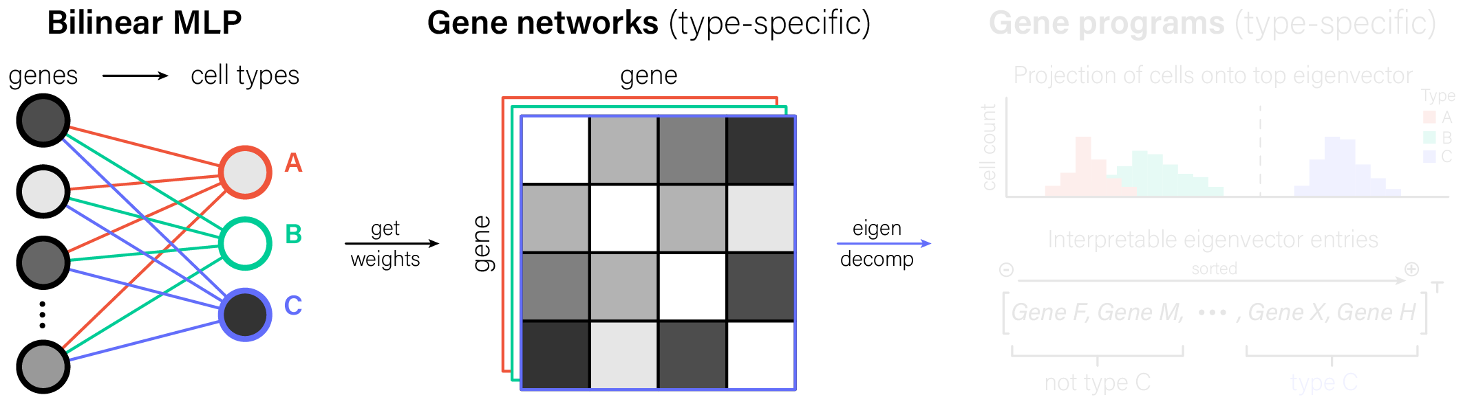
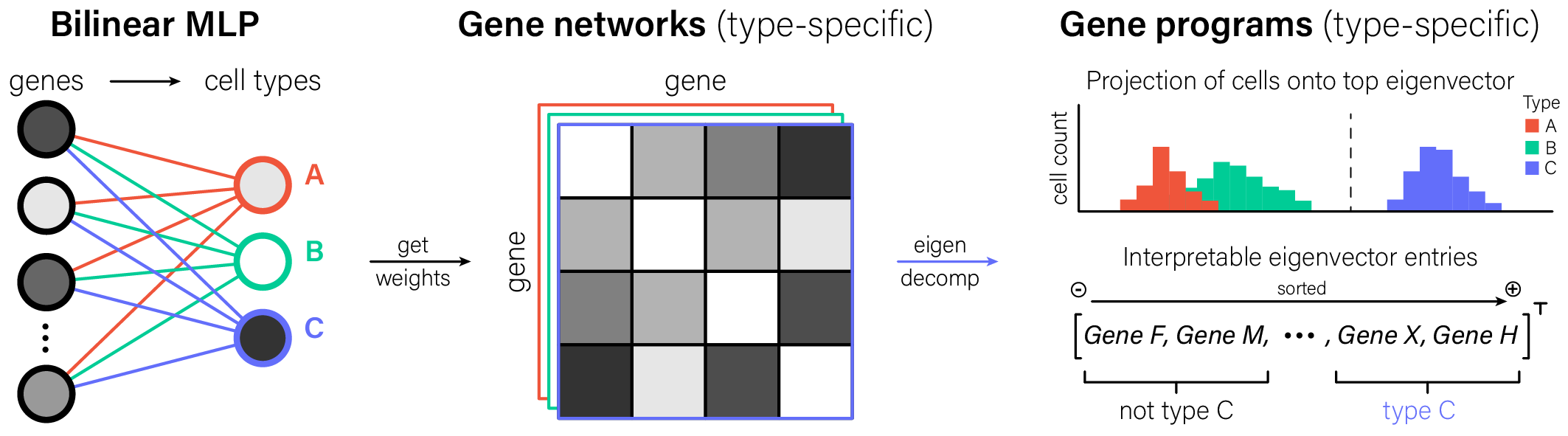
The key step in interpreting bilinear MLPs is seeing the weights for a given cell type output as a gene-gene graph. Once we have that graph, we can make the conventional single-cell transcriptomics move: eigendecompose its adjacency matrix to identify interpretable gene programs.
Let’s begin by defining our dimensions in terms of single-cell quantities.
- $g$: number of genes
- $h$: hidden dimension
- $t$: number of cell types
Weights $\mathbf{W}, \mathbf{V} \in \mathbb{R}^{h \times g}$ project from gene‑expression space into a hidden representation. An additional linear map $\mathbf{P} \in \mathbb{R}^{t \times h}$ then projects hidden features to $t$ cell‑type outputs. For simplicity we “fold” $\mathbf{P}$ into the weight matrices so they map directly from transcriptional space to cell‑type space.
\begin{equation} \mathbf{P} \mathbf{W} \rightarrow \mathbf{W} \in \mathbb{R}^{t \times g} \nonumber \end{equation} \begin{equation} \mathbf{P} \mathbf{V} \rightarrow \mathbf{V} \in \mathbb{R}^{t \times g} \nonumber \end{equation}
A bilinear layer computes
\begin{equation} g(\mathbf{x}) = \mathbf{W} \mathbf{x} \odot \mathbf{V} \mathbf{x}, \nonumber \end{equation}
where $\mathbf{x} \in \mathbb{R}^g$ is a cell’s transcriptional profile and the o-dot denotes elementwise multiplication. Bias terms are omitted here for conceptual clarity. Focusing on a single output (cell type) $a$, the expression becomes
\begin{equation} \mathbf{w}_a^{\top} \mathbf{x} \odot \mathbf{v}_a^{\top} \mathbf{x}. \nonumber \end{equation}
Each factor above is a scalar, so the elementwise product reduces to ordinary multiplication, and the left factor can equivalently be written as $\mathbf{x}^{\top}\mathbf{w}_a$. Applying these simplifications gives
\begin{equation} (\mathbf{x}^{\top} \mathbf{w}_a) (\mathbf{v}_a^{\top} \mathbf{x}). \nonumber \end{equation}
Expanding the product and defining the cell type–specific gene–gene interaction matrix \(\mathbf{Q}_a = \mathbf{w}_a \mathbf{v}_a^{\top} \in \mathbb{R}^{g \times g},\) we obtain the quadratic form
\begin{equation} \mathbf{x}^{\top} \mathbf{Q}_a \mathbf{x}. \nonumber \end{equation}
Only the symmetric part of $\mathbf{Q}_a$ contributes to $\mathbf{x}^{\top} \mathbf{Q}_a \mathbf{x}$, so we replace $\mathbf{Q}_a$ with \begin{equation} \frac{1}{2} (\mathbf{Q}_a + \mathbf{Q}_a^{\top}) \rightarrow \mathbf{Q}_a \nonumber \end{equation} and eigendecompose the resulting symmetric matrix for interpretation.
Only the symmetric part of $\mathbf{Q}_a$ contributes to $\mathbf{x}^{\top} \mathbf{Q}_a \mathbf{x}$
Since $\mathbf{Q}_a$ is square it decomposes into symmetric and antisymmetric parts. \begin{equation} \mathbf{Q}_a = \frac{1}{2} (\mathbf{Q}_a + \mathbf{Q}_a^{\top}) + \frac{1}{2} (\mathbf{Q}_a - \mathbf{Q}_a^{\top}) \nonumber \end{equation} The quadratic form $\mathbf{x}^{\top} \mathbf{Q}_a \mathbf{x}$ therefore decomposes in the same way. The symmetric contribution is \begin{equation} \frac{1}{2} \mathbf{x}^{\top} (\mathbf{Q}_a + \mathbf{Q}_a^{\top}) \mathbf{x} = \frac{1}{2} (\mathbf{x}^{\top} \mathbf{Q}_a \mathbf{x} + \mathbf{x}^{\top} \mathbf{Q}_a^{\top} \mathbf{x}). \nonumber \end{equation} and the antisymmetric part is \begin{equation} \frac{1}{2} \mathbf{x}^{\top} (\mathbf{Q}_a - \mathbf{Q}_a^{\top}) \mathbf{x} = \frac{1}{2} (\mathbf{x}^{\top} \mathbf{Q}_a \mathbf{x} - \mathbf{x}^{\top} \mathbf{Q}_a^{\top} \mathbf{x}). \nonumber \end{equation} Because $\mathbf{x}^{\top} \mathbf{Q}_a \mathbf{x}$ is a real scalar, \begin{equation} \mathbf{x}^{\top} \mathbf{Q}_a \mathbf{x} = (\mathbf{x}^{\top} \mathbf{Q}_a \mathbf{x})^{\top} = \mathbf{x}^{\top} \mathbf{Q}_a^{\top} \mathbf{x}, \nonumber \end{equation} and the antisymmetric contribution vanishes: \begin{equation} \frac{1}{2} (\mathbf{x}^{\top} \mathbf{Q}_a \mathbf{x} - \mathbf{x}^{\top} \mathbf{Q}_a^{\top} \mathbf{x}) = 0. \nonumber \end{equation} Therefore, only the symmetric part contributes.
The symmetric gene–gene interaction matrix $\mathbf{Q}_a$ can be read like a gene–gene covariance matrix in conventional single‑cell analysis. As with covariance, eigendecomposition of $\mathbf{Q}_a$ reveals prominent gene modules, but here those modules are directly tied to the model’s prediction of cell type $a$. Working with the symmetric part also simplifies interpretation because the spectral theorem guarantees real eigenvalues. The final step of interpretation is GO term analysis based on gene modules, the details of which are given below.
Cell type classification
Cell types in the developing pancreas
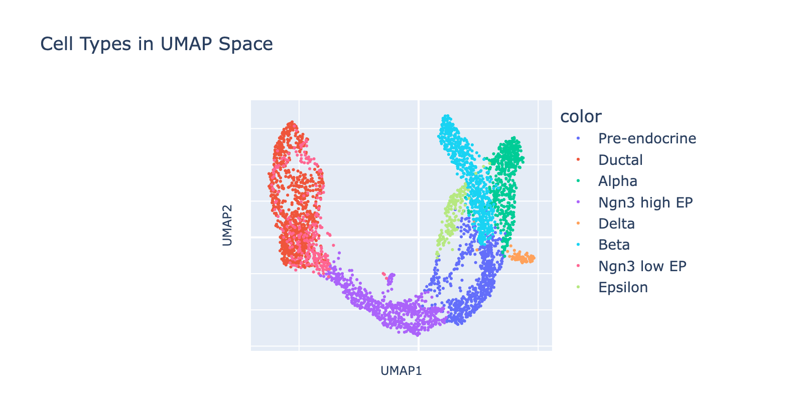
We start by training and interpreting a model on a straightforward task: cell type classification. The dataset is a collection of developing endocrine cells from the mouse pancreas with expert‑assigned cell type labels and continuous developmental structure that will be useful later.
First, we visualize the data in UMAP space colored by cell type (UMAP coordinates were precomputed by the scvelo package). The dominant developmental trajectory runs from ductal cells (left) to alpha and beta cells (right), with finer branching between epsilon/alpha and beta populations. In the next section we’ll quantify these nested transcriptional scales; here our goal is simply to predict cell types.
Model training {type}
To obtain interpretable $\mathbf{Q}_a$ matrices we trained a bilinear MLP on the pancreas data.
Training details
- Data:
scvelo.datasets.pancreas(); drop genes starting with Rpl/Rps; normalize total counts and apply log1p (use layerspliced). - Features: top 10,000 HVGs.
- Split: 70% train / 30% val (no test set; exploratory).
- Architecture: a single bilinear layer formed from two linear projections $\mathbf{W},\mathbf{V}$ (10k→128); their elementwise product feeds a linear head $\mathbf{P}$ producing $t$ cell‑type logits (see the interpretation section for mathematical details).
- Objective: cross‑entropy.
- Optimizer: Adam, lr = 1e‑4, weight decay = 0.35.
- Schedule: cosine annealing over 100 epochs.
- Batch size: 64.
- Device: CPU; seeds fixed (Python, NumPy, Torch) for reproducibility.
- Biases: biases were omitted to simplify downstream interpretation; this matches the original paper’s finding that biases had little effect on performance.
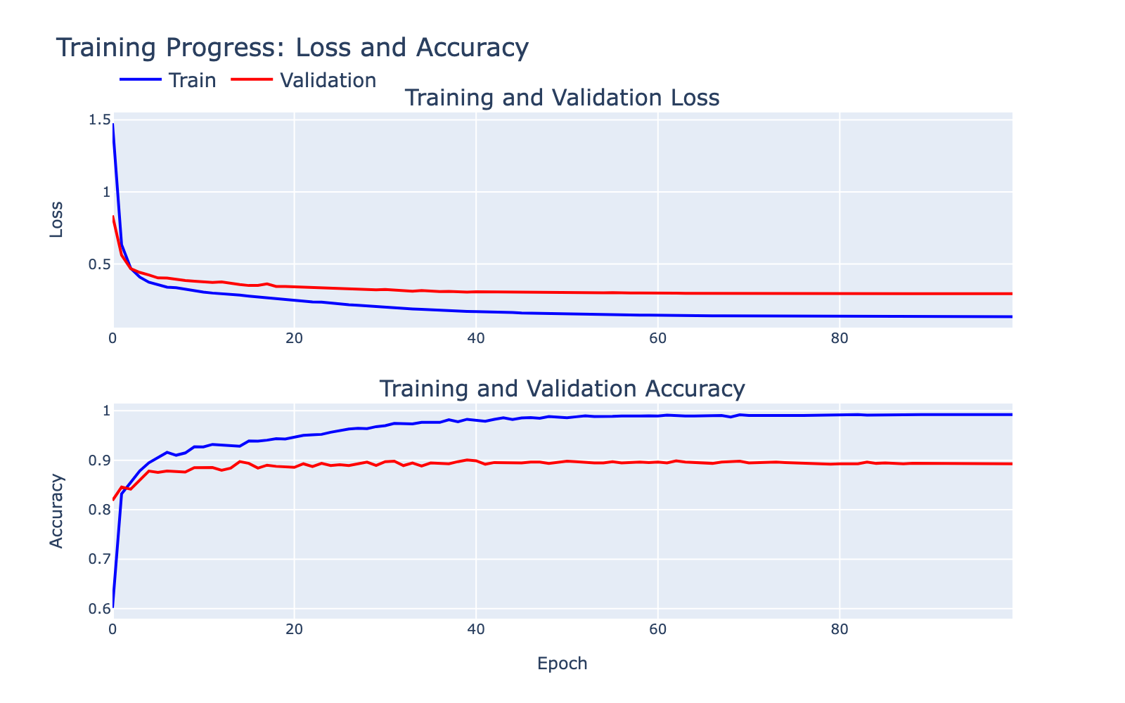
The training and validation loss/accuracy curves are shown below. There is a training/validation gap that indicates some overfitting, but the ~90% validation accuracy suggests the model captured meaningful signal worth inspecting. Note that the labels themselves are human annotations and may contain errors that limit achievable performance.
Overall, the classifier performed well enough that we expected it to have learned internal structure amenable to interpretation. Now let’s take a look at that structure.
Model interpretation {type}
We identify cell type-specific gene modules using the following interpretation pipeline:
- Extract per‑output interaction matrix $\mathbf{Q}_a$ and symmetrize to obtain a real, symmetric gene–gene matrix.
- Eigendecompose the symmetric matrix and select leading eigenvectors as gene modules.
- Project cells onto module axes to verify that module scores track the target (class label, frequency coordinate, or perturbation dose).
- Rank genes by loading per module sign and perform GO enrichment on top genes.
We walk through one cell type as an example. Results for a few other types are available in the dropdowns below.
Beta
Beta cells are the insulin‑secreting endocrine cells of the pancreas, marked by high expression of insulin genes (Ins1, Ins2) and regulators (Pdx1, Nkx6‑1). They preserve blood‑glucose homeostasis by releasing insulin in response to elevated glucose.
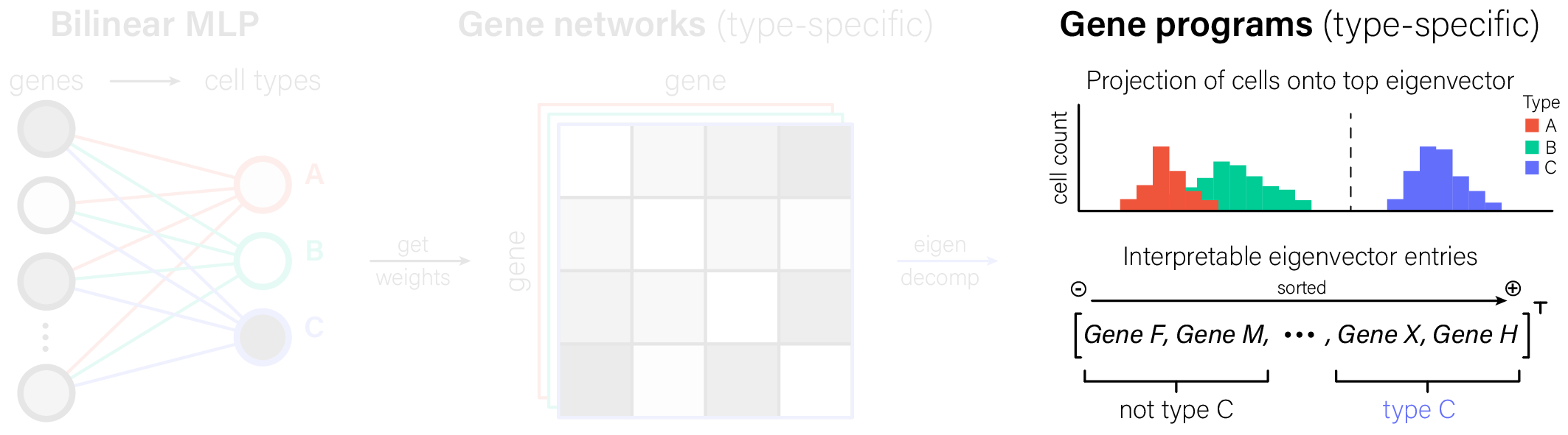
We expected the model to learn features that separate beta cells from other types, as we trained it on a classification task. To inspect these features, we project cells onto top gene modules (the eigenvectors of $\mathbf{Q}_{\mathrm{Beta}}$) and plot the distribution of module scores by cell type.
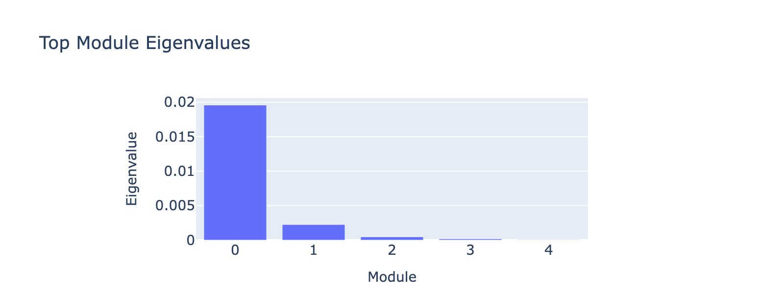
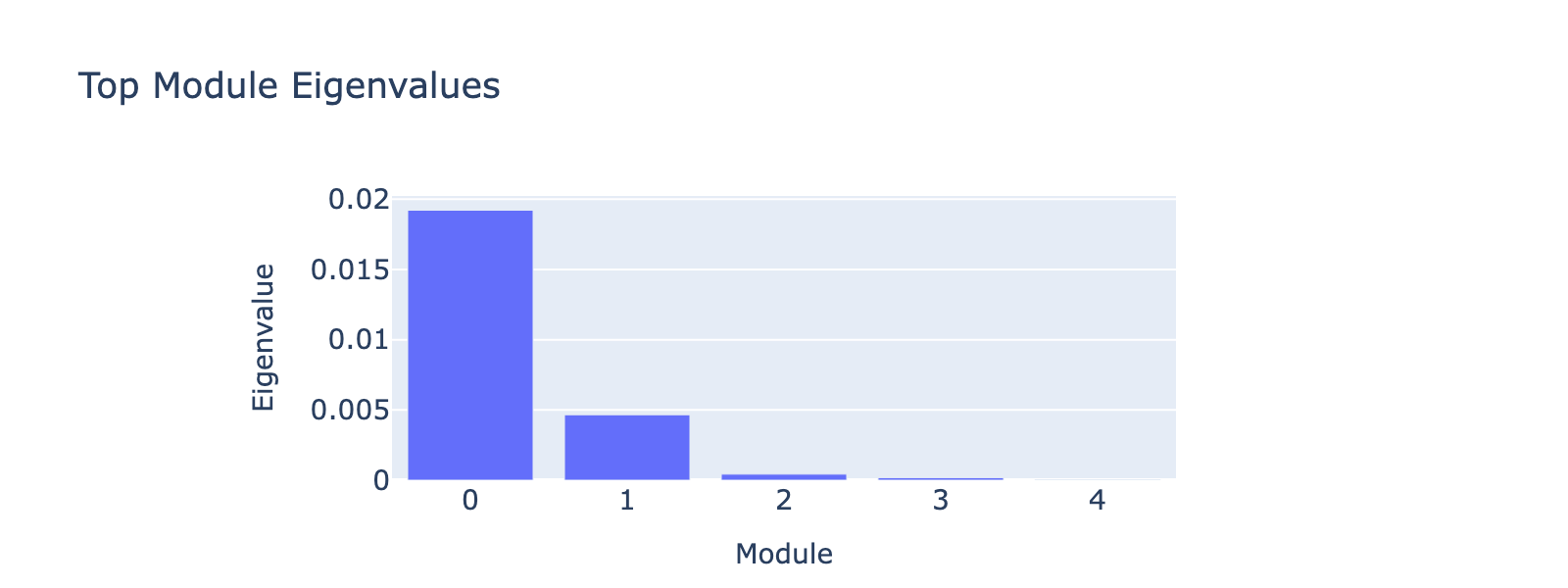
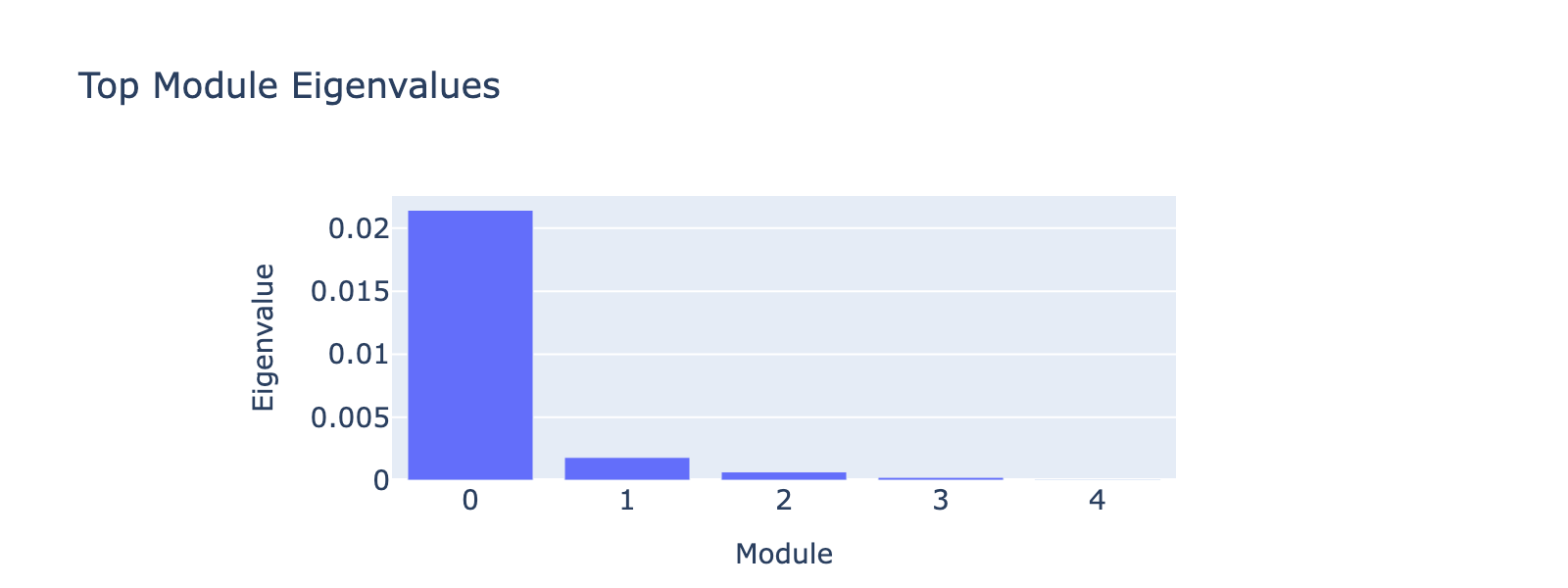
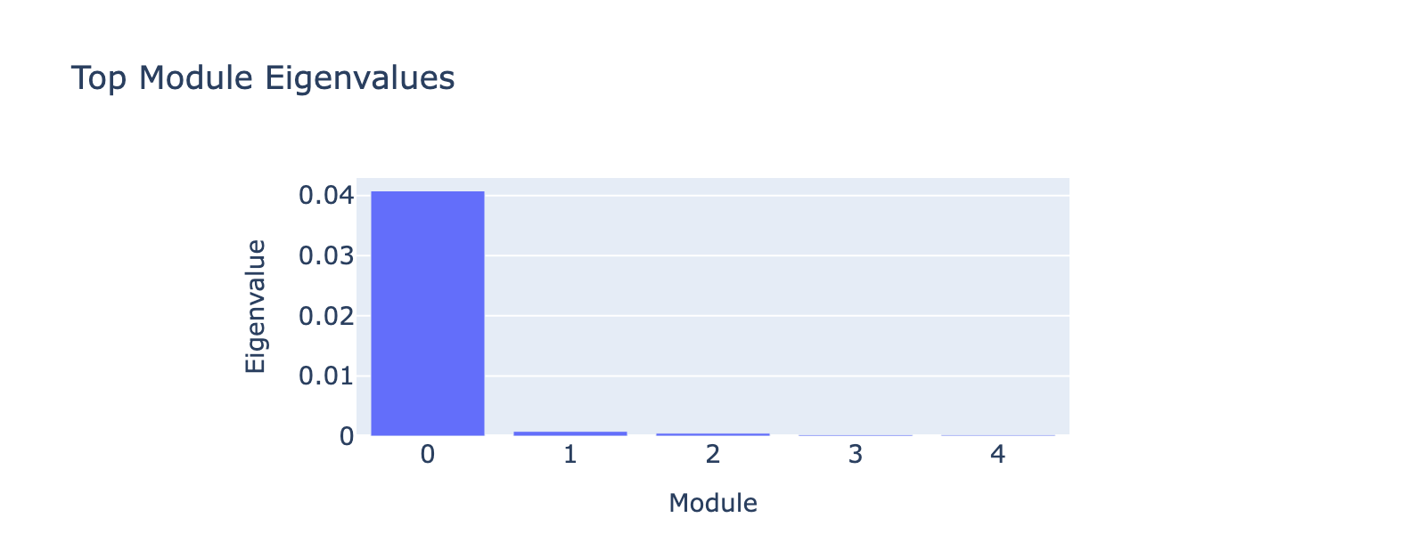
Before that, we have to decide how many top eigenvectors to inspect. Eigenvalues quantify module strength in the same way they do for PCA (variance explained), so we examine them to decide which modules merit interpretation.

The first eigenvalue dominates, so our biological interpretation focuses on the first module.
Now let’s plot histograms of cell projected onto module 0, separated by cell type. We’ll only visualize cells in the validation set to ensure our interpretations are transferrable. Module 0 clearly separates beta cells from the rest (blue cluster on the right).
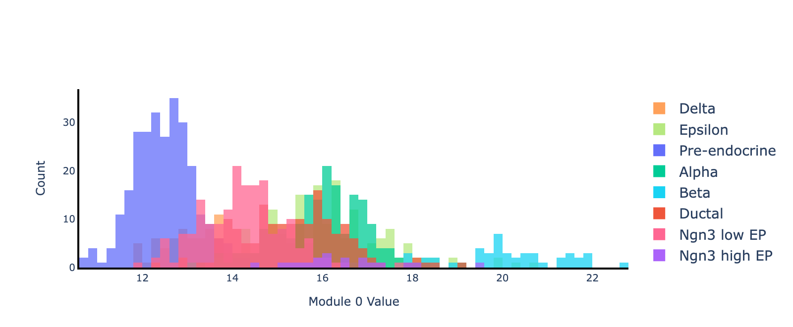
Note that the sign of an eigenvector is arbitrary (multiplying by $−1$ yields another valid eigenvector), so only the separation between cell types matters, not which are more “positive” or “negative.”
Ok, so we’ve observed that the model is capable of separating cell types based on modules. But on what basis is it separating cells? This is where the eigenvectors come in – they describe a linear projection into gene space that is evidently capable of classifying cells. Due to the linearity, all we need to do is inspect entries with extreme values, as they represent the gene weights that determine .
GO term analysis details
- Gene ranking: select the top 1% of genes per sign (100 genes per sign out of 10,000 HVGs). Signs are treated as opposite poles on a one‑dimensional axis, not as intrinsic activators/repressors; we refer to these lists as gene programs (“positive program” / “negative program”).
- GO enrichment: run over‑representation analysis via Enrichr (gseapy) using:
GO_Biological_Process_2023,GO_Molecular_FUNCTION_2023,GO_Cellular_COMPONENT_2023,KEGG_2019_Mouse,Reactome_2022,MSigDB_Hallmark_2020,WikiPathways_2019_Mouse(organism="mouse"). We keep terms with Benjamini–Hochberg adjusted $p \leq 0.05$ and display the top 15 by adjusted $p$. No further manual pruning was applied beyond the earlier removal of Rpl/Rps genes prior to HVG selection. (Caveat: Enrichr results depend on gene‑list size and background; interpret enrichments as hypotheses and examine redundancy/overlap among enriched terms.) - Interpretation limits: interactions in quadratic weights reflect statistical associations used for prediction, not demonstrated causal regulation. GO results compound hypothesis layers (gene selection + eigenvector choice), so we treat annotations as hypotheses that require experimental validation.
This workflow produced the following for module 0:
Overall interpretation
- Positive side: canonical insulin / β‑cell lineage program (Pancreas β Cells, MODY, FoxO signaling, insulin secretion, glucose homeostasis) with metabolic and cell‑cycle regulators (Nnat, Ins1, Ins2, Pdx1, Nkx6‑1, Mafb, G6pc2, Slc30a8). Moderate cell‑cycle and FoxO/AMPK signals suggest metabolically active differentiating β cells balancing proliferation and functional maturation.
- Negative side: polyhormonal / secretory stress and ER remodeling (secretory granule lumen, peptide hormone metabolism, ER processing, degranulation, chaperones, mTORC1) with inflammatory/apoptotic signatures consistent with a mixed, stress‑buffering endocrine state and broad vesicle biogenesis.
- Comparison: a contrast between insulin‑focused maturation (positive) and a broader stress/adaptive secretory program (negative), reflecting resolution from polyhormonal stress buffering to β functional consolidation.
Top 10 genes
- Positive: Nnat, Pdx1, Ins2, Gng12, Mafb, Ins1, Dlk1, Nkx6‑1, Ociad2, Hadh
- Negative: Ghrl, Cdkn1a, Cck, Malat1, Neurog3, Peg3, Maged2, Eef1a1, Gcg, Isl1
Key GO terms
- Positive: Pancreas Beta Cells; Maturity Onset Diabetes of the Young; Regulation of Insulin Secretion; FoxO Signaling; Cellular Response to Glucose
- Negative: Secretory Granule Lumen; Peptide Hormone Metabolism; Protein Processing in ER; Platelet Degranulation; mTORC1 Signaling
Thus, module analysis reveals that the model represents beta cells using canonical marker programs — a useful sanity check and proof of concept.
Additional examples
Results for other cell types and their top modules are available in the dropdowns below.
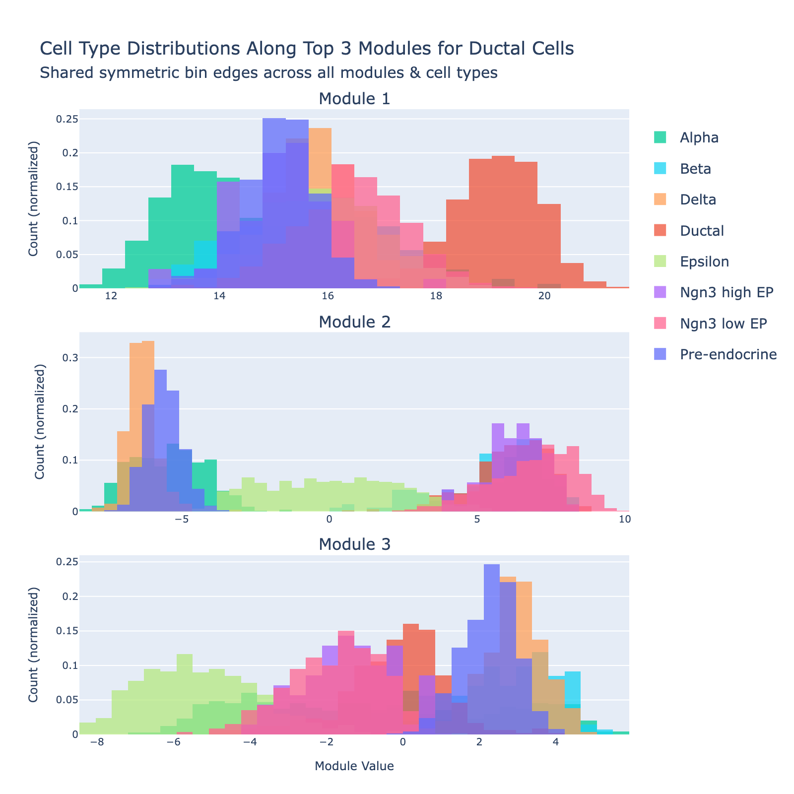
Ductal
Ductal cells are the epithelial cells that line the pancreatic ductal tree. During endocrinogenesis they provide a tubular scaffold and act as a progenitor/support niche and signaling source for emerging endocrine cells.
Overall interpretation
- Positive side: developmental / progenitor and early endocrine specification program combining transcriptional regulators (Pdx1, Hhex, Sox4), morphogen/secreted factors (Ghrl, Sst, Enho), and epithelial/surface markers (Cd24a, Prrg2). Sparse classical secretory granule machinery suggests a less terminally differentiated duct‑associated / progenitor‑leaning population retaining endocrine lineage priming.
- Negative side: mature endocrine / secretory granule and peptide hormone module enriched for polyhormonal cargo (Gcg, Pyy, Iapp, Gast, Cpe, Ttr) plus metabolic/signaling scaffolds (Gnas, Malat1). GO terms highlight ER protein processing, vesicle/granule lumen, platelet (secretory) degranulation, and peptide hormone metabolism—typical of active secretory endocrine cells.
- Comparison: separates regulatory priming/developmental transcriptional control (positive) from established multi‑hormone secretory function (negative).
Top 10 genes
- Positive: Ghrl, Cd24a, Npepl1, Sst, Pdx1, Enho, Hhex, Prrg2, Sox4, Mdk
- Negative: Gcg, Pyy, Ttr, Tmem27, Gnas, Malat1, Arx, Cpe, Iapp, Gast
Key GO terms
- Positive: Maturity Onset Diabetes of the Young (developmental TFs); Pancreas Beta Cells (early regulators); Cellular Response to Glucose; Insulin Secretion (early priming)
- Negative: Pancreas Beta Cells; Protein Processing in ER; Peptide Hormone Metabolism; Platelet/Secretory Degranulation; Gap Junction
Ngn3 high EP
Ngn3‑high endocrine progenitors (Ngn3‑high EP) are a transient, rare population marked by high expression of Neurog3. These committed endocrine precursors are transcriptionally immature and plastic, enriched for developmental programs (Notch/Delta and lineage TFs), often show proliferative signatures, and will differentiate into hormone‑producing endocrine cell types (α, β, δ, etc.).
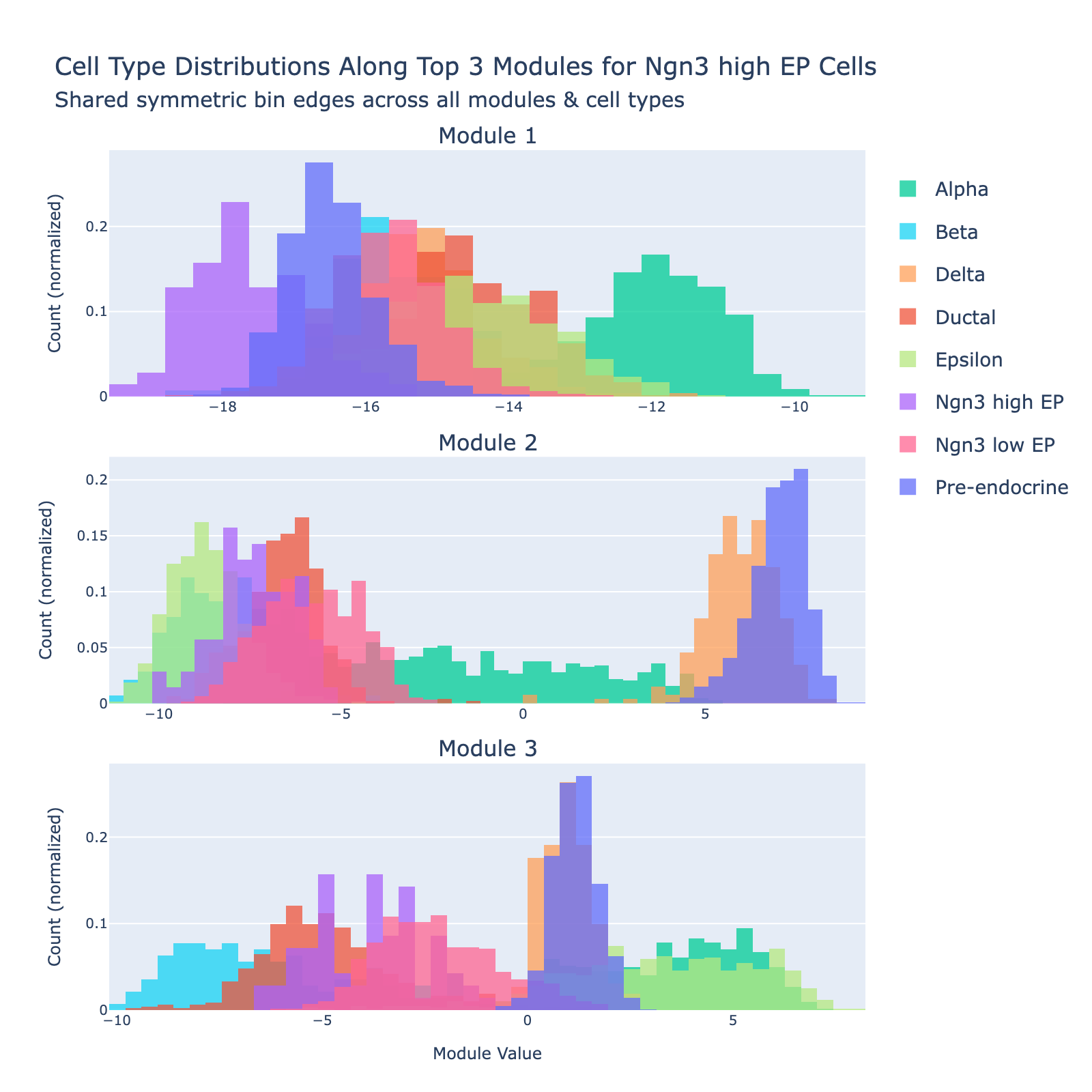
Overall interpretation
- Positive side: Notch / endocrine progenitor & cell‑cycle signaling (Neurog3, Arx, Amotl2, Cited4, Rasd1) with Rho/chromatid cohesion and Delta‑Notch enrichment—captures specifying endocrine precursors before strong secretory specialization.
- Negative side: broad ER/secretory stress and hormone activity (protein processing ER, cAMP signaling, secretory/vesicle lumen, mTORC1, TNF‑α via NF‑κB) featuring mature peptide handling (Sst, Pyy, Ttr, Ghrl), chaperones (Hspa5, Calr), and metabolic scaffolds (Gnas, Aldoa, Gapdh).
- Comparison: early endocrine commitment and proliferation (positive) versus established secretory/ER expansion and stress adaptation (negative).
Top 10 genes
- Positive: Neurog3, 8430408G22Rik, Amotl2, Gcg, Tmem171, Cited4, Arx, 2010107G23Rik, Rasd1, Gast
- Negative: Sst, Rbp4, Pyy, Hhex, Dlk1, Cd24a, Malat1, Eef1a1, Isl1, Iapp
Key GO terms
- Positive: Delta‑Notch Signaling; Regulation of β‑Cell Development; Mitotic Spindle / G2‑M Checkpoint; Pancreas Beta Cells (early TFs)
- Negative: Protein Processing in ER; Thyroid Hormone Synthesis; cAMP Signaling; Hormone Activity; mTORC1 Signaling
Alpha
Alpha cells are defined by high expression of glucagon (Gcg) and lineage determinants such as Arx; they raise blood glucose through glucagon secretion.
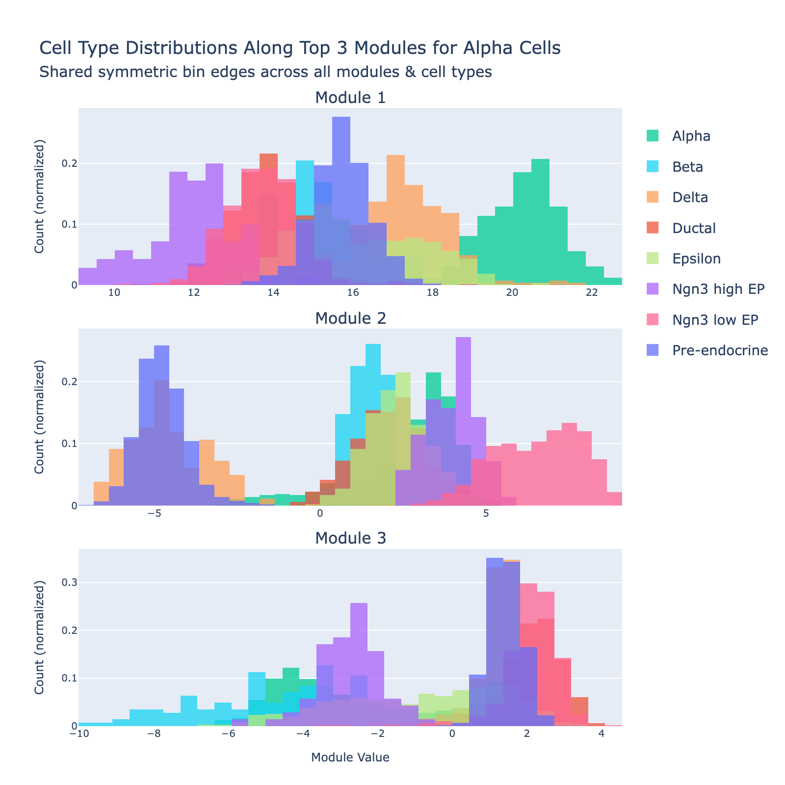
Overall interpretation
- Positive side: early endocrine lineage specification and stress/platelet degranulation signaling mixed with transcriptional control (Neurog3, Pax4, Nkx6‑1, Insm1), calcium/vesicle release (Cd63, Pfn1, Calm1), and apoptosis/p53 response (Cdkn1a, Btg2).
- Negative side: mixed metabolic stress, proliferation, and remodeling (apoptosis, TNF‑α, AMPK, UV response, Myc targets) with reduced classic secretory peptides.
- Comparison: specification/progenitor program (positive) versus adaptive stress/proliferative remodeling (negative).
Top 10 genes
- Positive: Neurog3, Eef1a1, Malat1, Cd63, Tmsb4x, Mdk, Cdkn1a, Btg2, Gnas, Cyb5r3
- Negative: Sst, Hhex, Ccnd1, Iapp, Deb1, Atp1b1, Meis2, Psat1, Hpgd, Cyr61
Key GO terms
- Positive: Regulation of β‑Cell Development; Platelet / Secretory Degranulation; Pancreas Beta Cells (specification factors); Apoptosis; Maturity Onset Diabetes of the Young
- Negative: Apoptosis; TNF‑α Signaling via NF‑κB; Unfolded Protein Response; AMPK Signaling; Maturity Onset Diabetes of the Young (late differentiation subset)
Summary {type}
We trained a reasonably accurate cell type classifier (~90% validation accuracy, with some overfitting) and eigendecomposed $\mathbf{Q}_a$ to extract gene modules that the model uses to recognize cell type $a$. GO analysis shows these modules separate cell types in a one‑versus‑all fashion using gene programs that align with established biology. Compared with standard post‑hoc approaches (e.g., t‑tests), this method yields direct, parameter‑based markers for each class.
Because supervised cell typing depends on human labels (which can be biased or noisy), we next explore learning analogous properties that come directly from the data itself — for example, transcriptional frequencies.
Frequency regression
From the UMAP above we can see that the transcriptional landscape is dominated by a long developmental trajectory running from naive ductal cells to mature alpha/beta/epsilon/delta populations. Smaller, nested patterns also exist (for example, differences among mature endocrine types). This intuition motivates a notion of transcriptional “scale” that we formalize as transcriptional “frequencies.” Analogous to temporal frequencies in music which describe pressure variation on different time scales, transcriptional frequencies describe cellular variation on different transcriptomic scales. Importantly, frequencies capture structure directly from the data rather than relying on human labels.
Mathematically this is most easily framed using graph signal processing, which in practice reduces to eigendecomposition of a transcriptional similarity graph. Concretely, we build a k‑nearest‑neighbors graph over cells to get an adjacency matrix
\[\mathbf{A} \in \mathbb{R}^{n \times n},\]where $n$ is the number of cells. This graph defines a “transcriptional domain” in which distance (or scale) is measured by graph hops. Frequencies are the eigenvectors of the graph Laplacian
\[\mathbf{L} = \mathbf{D} - \mathbf{A},\]where $\mathbf{D} \in \mathbb{R}^{n \times n}$ is the diagonal degree matrix. One reason to prefer the Laplacian over the raw adjacency is that its eigenvalues are non‑negative, which matches our usual intuition that frequencies should be non‑negative. For more background and examples see this post about spatial frequencies over tissues.
These frequencies are closely related to diffusion components. They differ mainly by matrix normalization choices. We use the frequency perspective because it ties cleanly to signal‑processing intuition and is often more intuitive when reasoning about scales of variation.
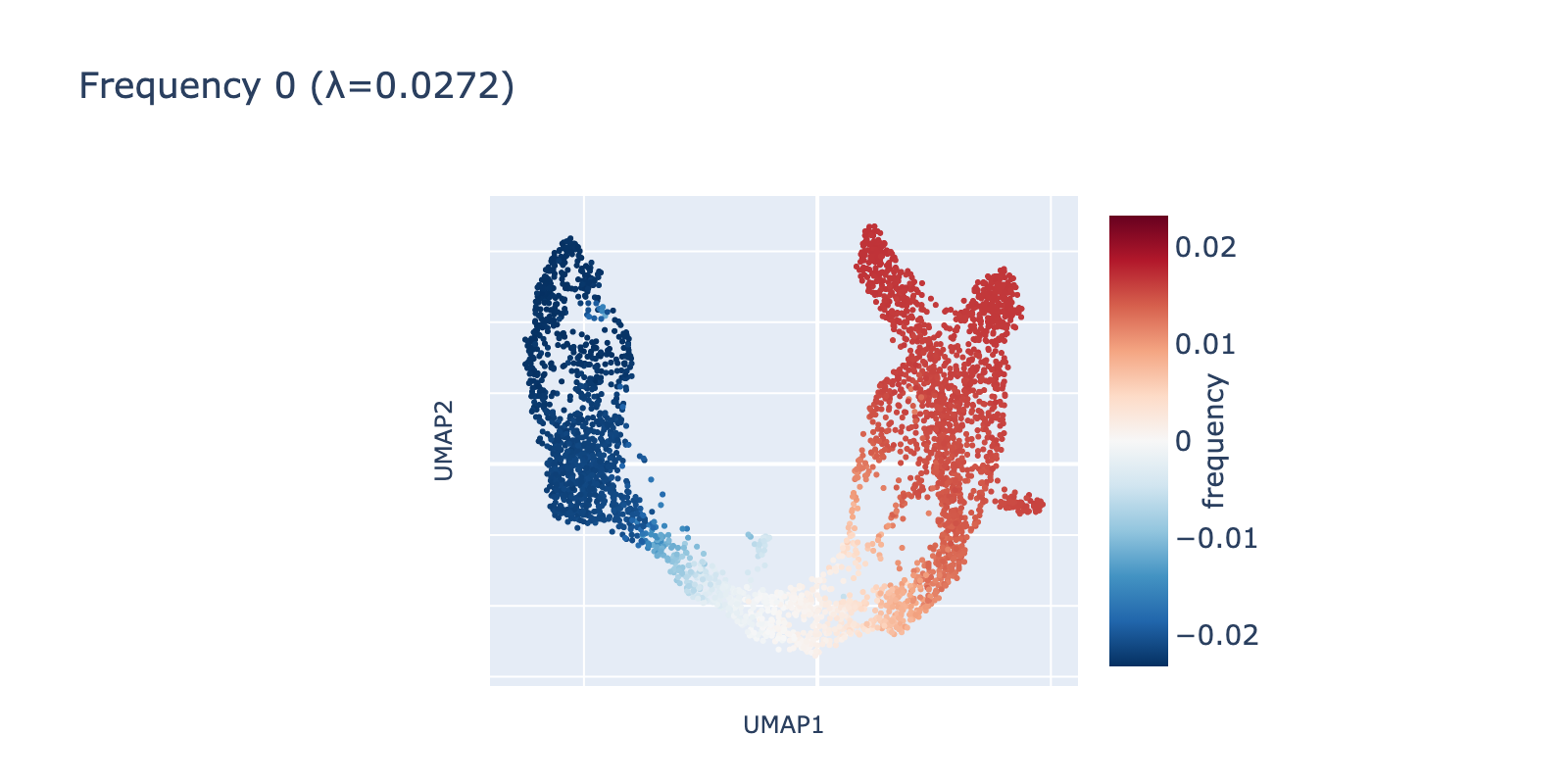
Transcriptional frequencies in the developing pancreas
We visualized the leading frequencies to check whether they capture interpretable patterns. The lowest frequency (eigenvalue $\lambda=0.272$) runs along the same long developmental axis described above: naive cells have negative values, mature cells positive values, and transitional cells lie between. In other words, this frequency captures the largest, most consistent transcriptomic difference in the dataset.
The second frequency appears visually higher (it oscillates along the same axis), going low→high→low across the trajectory. A simple analogy is comparing a single‑period sine wave to one with 1.5 periods compressed into the same interval.
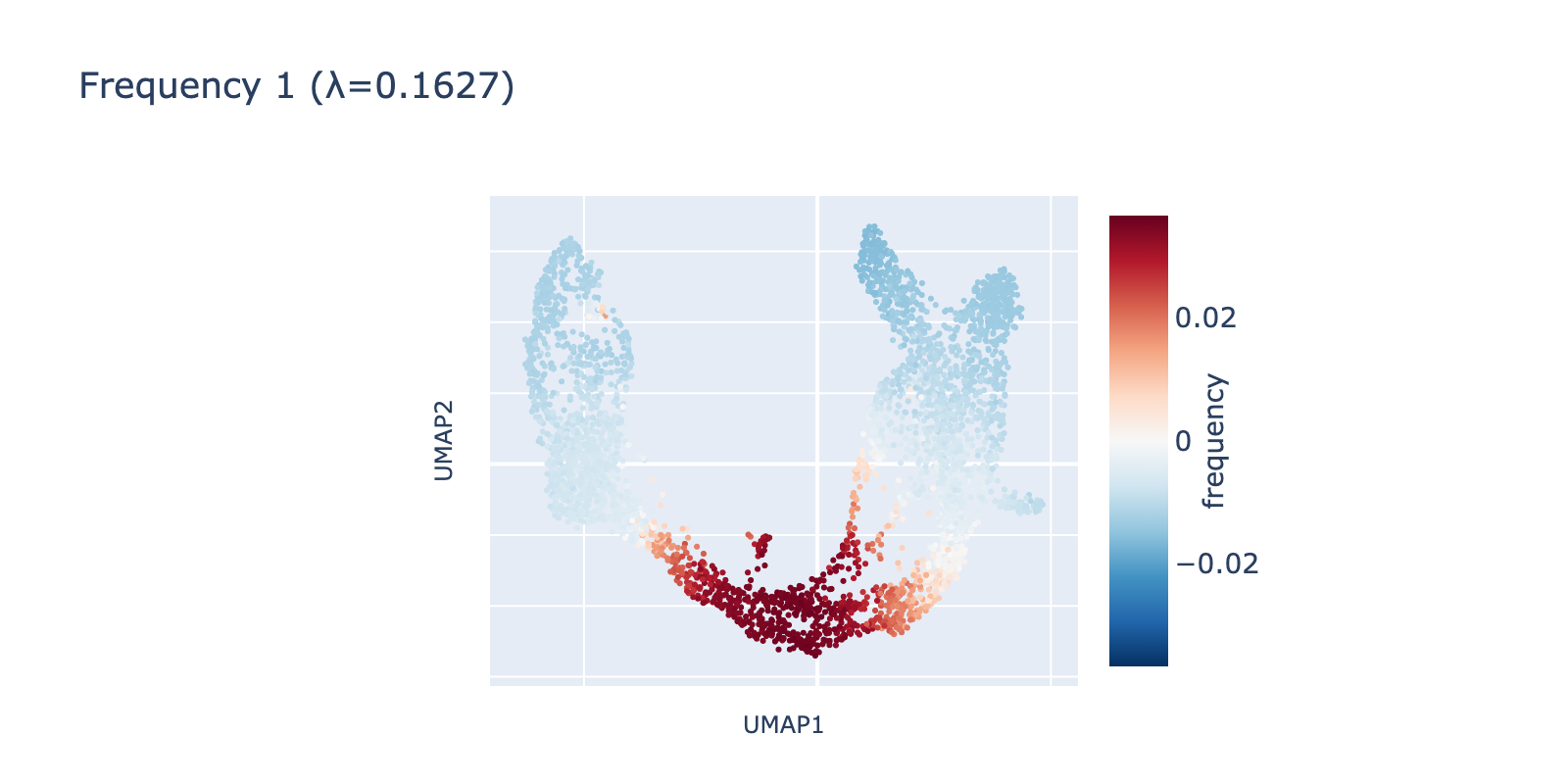
Because frequency 1 is prominent, it likely reflects a real biological signal rather than noise. One plausible interpretation is that it highlights a proliferative or transient state present in dividing cells but absent in more stable ductal or mature populations.
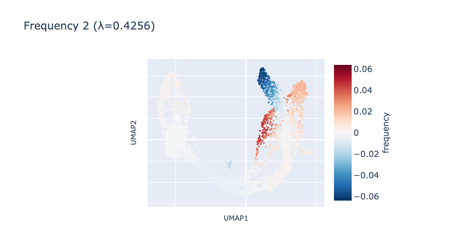
Frequency 2 captures a smaller, more localized fluctuation restricted to branches of the transcriptional manifold and appears to separate mature β cells from α/δ/ε cells—a subtler pattern than the first two frequencies.
Frequency 3 looks noisier: it contains a faint large‑scale fluctuation among naive cells and a small, distinct negative group branching from the center.
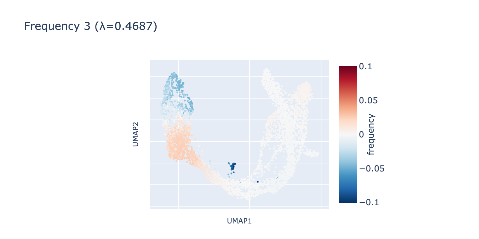
Although there are as many frequencies as there are cells (the Fourier transform here is a rotation into a frequency space of equal dimension), we focus our analysis on the first three frequencies. Smaller components can be real signals, but they tended not to align with expert cell‑type annotations in this dataset, so we omit them for clarity.
Whereas cell typing partitions cells into discrete classes, frequencies reveal nested continuous relationships. Thus, a model’s performance on a frequency output measures how well it captures a cell’s coordinate along that transcriptional scale (e.g., naive→mature or beta→alpha), not how well it isolates a single class.
Model training {freq}
Training was the same as for cell typing except for the regression objective and a few optimizer/architecture choices:
- Data:
scvelo.datasets.pancreas(); remove genes starting with Rpl/Rps; normalize total + log1p (layerspliced). - Features: top 10,000 HVGs.
- Split: 70% train / 30% val; no test set (exploratory).
- Architecture: bilinear layer; two linear projections $\mathbf{W},\mathbf{V}$ (10k→128) whose element‑wise product feeds a linear head $\mathbf{P}$ to $f$ frequency values.
- Objective: Huber loss (more robust to outliers than MSE or L1).
- Optimizer: Adam, lr = 1e‑4, weight decay = 1e‑4.
- Schedule: cosine annealing over 100 epochs.
- Batch size: 64.
- Device: CPU; seeds fixed (Python, NumPy, Torch) for reproducibility.
- Biases: biases were omitted to simplify downstream interpretation; this matches the original paper’s finding that biases had little effect on performance.
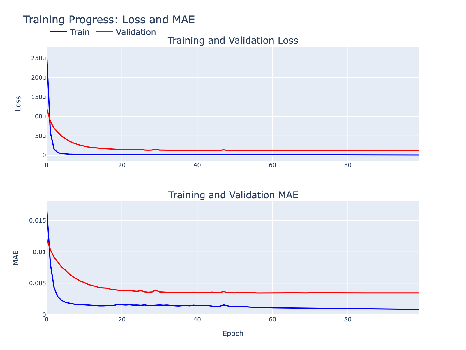
Overfitting was minimal for our exploratory goals. Below are supplementary model diagnostics.
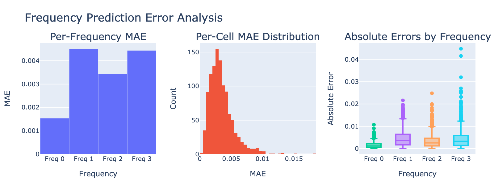
Validation MAE values are numerically small but should be interpreted in the context of each frequency’s distribution. Because these distributions are not Gaussian, directly comparing the MAE to the standard deviation is inappropriate. Instead, we visualize model performance by plotting module scores against frequency values (plots below), which gives a more intuitive sense of how well modules track each frequency.
Model interpretation {freq}
As with cell types, we focus on one output dimension in depth and leave other examples in dropdowns. We applied the same biological interpretation workflow used for cell typing.
Frequency 0
Rather than plotting module histograms by class, we plot module scores against frequency values — this is natural for a regression task, since module scores should predict frequency coordinates. Coloring points by cell type provides an additional biological sanity check.
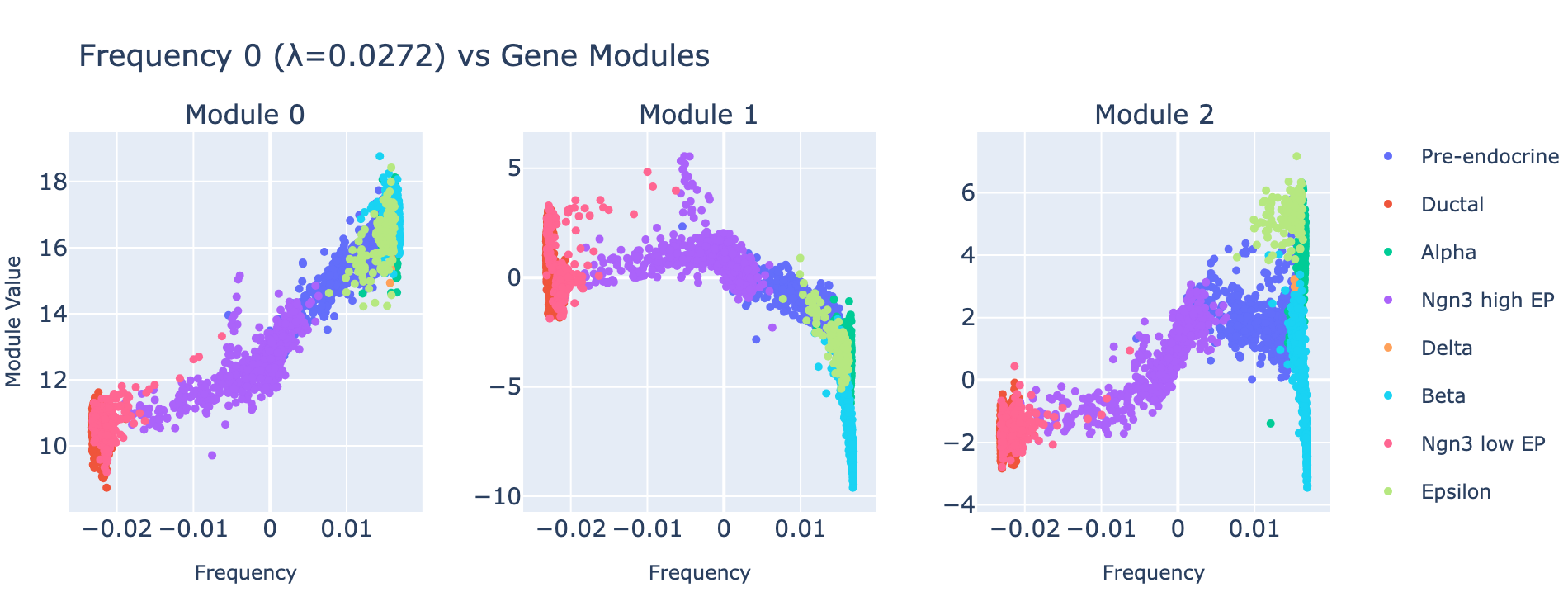
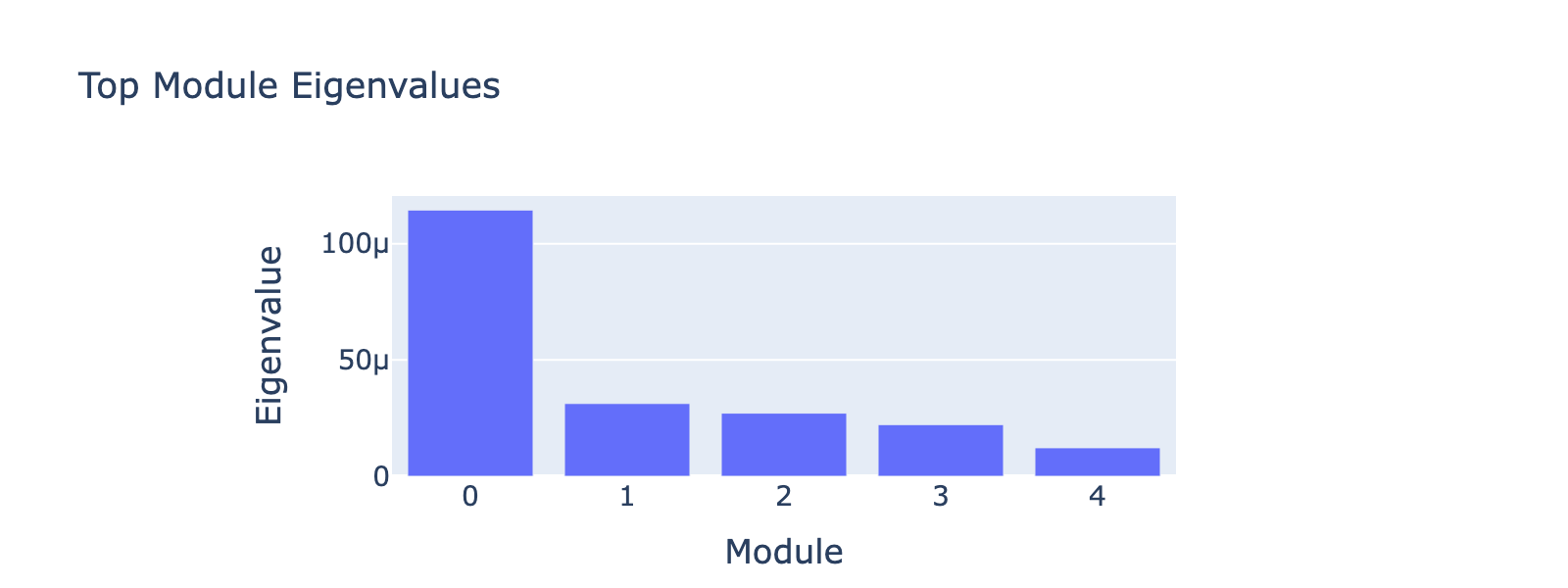
Module 0 correlates tightly with frequency 0, and the ordering of cell types along this axis matches the developmental trajectory (ductal → differentiated endocrine). Subsequent modules capture aspects of the same progression but with weaker signal. The eigenvalues confirm module 0 is the dominant contributor.
Examining the genes that load on module 0 yields biologically coherent programs.
Overall interpretation
- Positive side: canonical endocrine secretory and peptide hormone programs (Pancreas β cell set; hormone activity; regulation of insulin secretion; peptide hormone metabolism). Top genes (Malat1, Gnas, Pcsk1n, Cpe, Pfn1, Rbp4, Iapp, Pyy, Dynll1, Aplp1) include components for insulin granule processing, endocrine peptides, signaling scaffolds, and cytoskeletal transport—consistent with a mature secretory phenotype.
- Negative side: extracellular matrix / structural and developmental genes (collagen‑containing ECM, ER lumen) such as (Gas6, Cd24a, Sox9, Csrp1, Col9a3, Bicc1, Lamb1) indicative of progenitor/ductal or less differentiated states.
- Comparison: defines a differentiation axis contrasting mature secretory endocrine identity with progenitor/ECM remodeling.
Top 10 genes
- Positive: Malat1, Gnas, Pcsk1n, Cpe, Pfn1, Rbp4, Iapp, Pyy, Dynll1, Aplp1
- Negative: Gas6, Cd24a, Sox9, Csrp1, Col9a3, Bicc1, Rbp2, Lamb1, Maob, Pi4k2b
Key GO terms
- Positive: Pancreas β Cells; Hormone Activity; Regulation of Insulin Secretion; Peptide Hormone Metabolism; Secretory Granule Degranulation; Neuropeptide Hormone Activity
- Negative: Collagen‑Containing Extracellular Matrix; Urogenital System Development
In sum, the model represents nonlinear transcriptional frequencies using interpretable gene modules that align with known biology.
Additional examples
Frequency 1
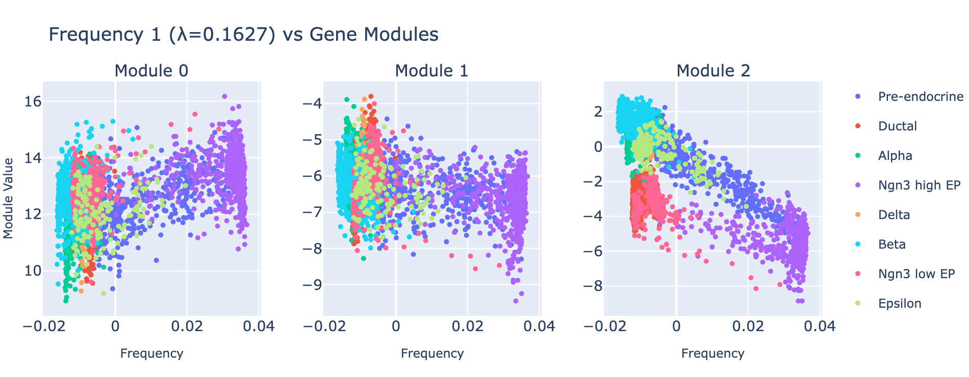
Overall interpretation
- Positive side: ER/protein folding and adaptive stress signature (Protein Processing in ER, Unfolded Protein Response, ATF6) coupled with cytoskeletal/junctional remodeling and early endocrine specification.
- Negative side: protease/endopeptidase and ubiquitin ligase binding terms plus hormone activity, suggesting a secretion‑biased proteostasis state.
- Comparison: contrasts early UPR‑driven biosynthetic ramp‑up with more homeostatic, secretion‑focused states.
Top 10 genes
- Positive: Hspa5, Tuba1a, Epcam, Jun, Ssr2, Cd81, Tubb5, Cdk4, Ier2, Pdia6
- Negative: Eef1a1, Arf5, Hsp90aa1, Ngfrap1, Gabarapl2, Eif4a2, Clps, Slc25a5, Gcg, Krt18
Key GO terms
- Positive: Protein Processing in Endoplasmic Reticulum; Unfolded Protein Response; Pancreas β Cells; RHO GTPases Activate ROCKs; Tight Junction
- Negative: Endopeptidase Activity; Ubiquitin Protein Ligase Binding; Hormone Activity
Frequency 2
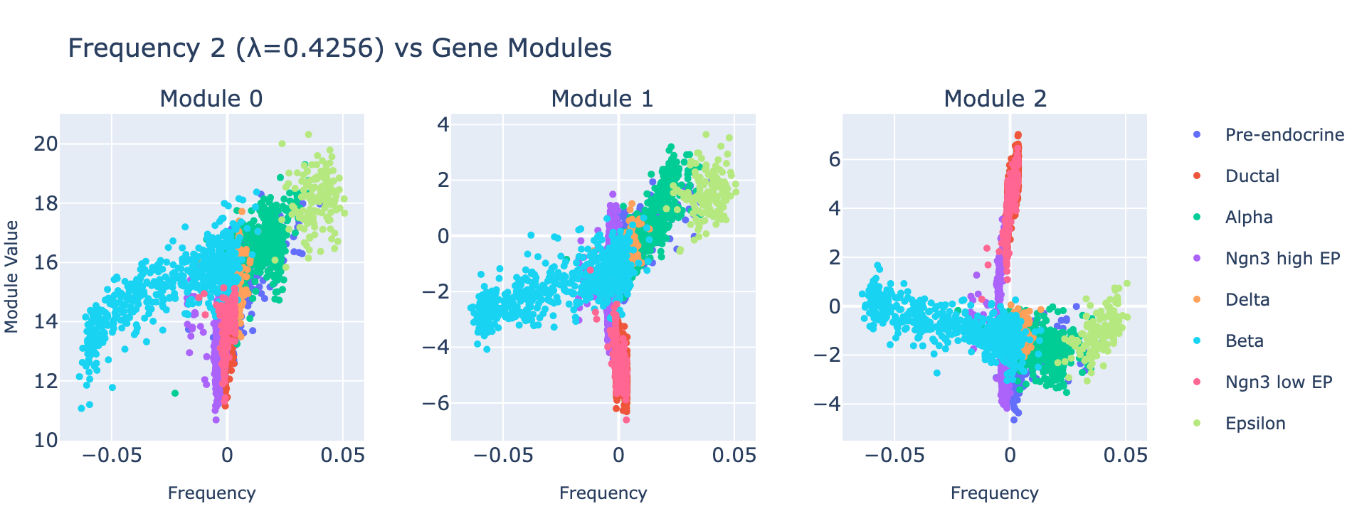
TODO: revisit this note. Note that the trend is evident across alpha, beta, and epsilon cells, yet earlier ductal and Ngn3 cells are fixed at a lower module value. This might be cleaned up by including a bias term in the bMLP layer, which we omitted for simplicity in this post.
Overall interpretation
- Positive side: broad multi‑hormone secretory program with ER folding/antigen processing and cytoskeletal maturation—consistent with a polyhormonal/transitional endocrine state.
- Negative side: insulin‑lineage maturation and glucose‑responsive programs marking specialized β cells.
- Comparison: contrasts polyhormonal transitional identities with insulin‑specialized mature β programs.
Top 10 genes
- Positive: Ghrl, Gcg, Rbp4, Isl1, Pfn1, Ssr2, Malat1, Iapp, Ngfrap1, Ttr
- Negative: Ins2, Ins1, Npy, Adra2a, Nnat, Gip, Sytl4, Spock2, Scaper, Mapt
Key GO terms
- Positive: Protein Processing in Endoplasmic Reticulum; Peptide Hormone Metabolism; Secretory Granule Lumen; mTORC1 Signaling; Antigen Processing and Presentation
- Negative: Maturity Onset Diabetes of the Young; Regulation of Insulin Secretion; Insulin Secretion; Type B Pancreatic Cell Differentiation
Summary {freq}
Frequencies provide a principled way to quantify transcriptional scales (analogous to diffusion components). Bilinear MLPs can learn to predict a cell’s coordinate in this frequency space and, at the same time, produce explicit gene modules (via eigendecomposition) that mark each frequency. These parameter‑based markers are more directly transferable between datasets than eigendecomposition‑based components alone. Additionally, weights-based interpretation offers direct gene markers for a given frequency, unlike conventional post-hoc marker analysis for diffusion components which is based on correlation with individual genes.
Although frequency and cell‑type tasks are complementary, perturbation regression (next) better exploits the causal and continuous aspects of bilinear MLPs and therefore may reveal richer biological insights.
Perturbation regression
TODO: only keep first module; omit additional components
Single-cell perturbation experiments profile how individual cells respond to genetic or chemical perturbations, enabling stronger causal claims about regulatory programs than observational atlases alone. Many current approaches optimize predictive accuracy at the expense of mechanistic transparency. For example, deep latent‑variable or discriminative methods such as scGen can perform well but do not expose explicit gene–gene mechanisms. By contrast, bilinear MLPs yield per‑output gene–gene interaction matrices whose symmetric eigendecomposition produces direct, parameter‑based gene programs that balance interpretability and predictive power. Here we treat perturbation prediction as a regression task to capture continuous, dose‑scaled effects and use bilinear MLPs to extract interpretable gene–gene modules for each perturbation.
Perturbation dataset
The dataset contains A549 cells (human lung adenocarcinoma) exposed to four different compounds. The original study introduced a high‑throughput perturbation and RNA‑sequencing workflow profiling hundreds of thousands of cells. Because the study reported distinct transcriptional effects across perturbations, it suited our proof‑of‑concept analysis.
Preprocessing was required. Low‑count cells formed mixed perturbation clusters, so we removed cells with fewer than 5k counts. This reduced the dataset from ~25k to ~10k cells but produced cleaner data, improved model fit, and more reliable interpretations.
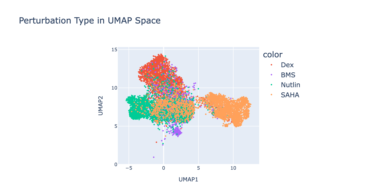
Perturbations are largely separable in UMAP space. SAHA shows the clearest dose‑dependent branching to the right with increasing dose. Nutlin shows a similar trend toward the left. BMS branches downward, but only at lower doses. Dex trends upward with no clear dose pattern.
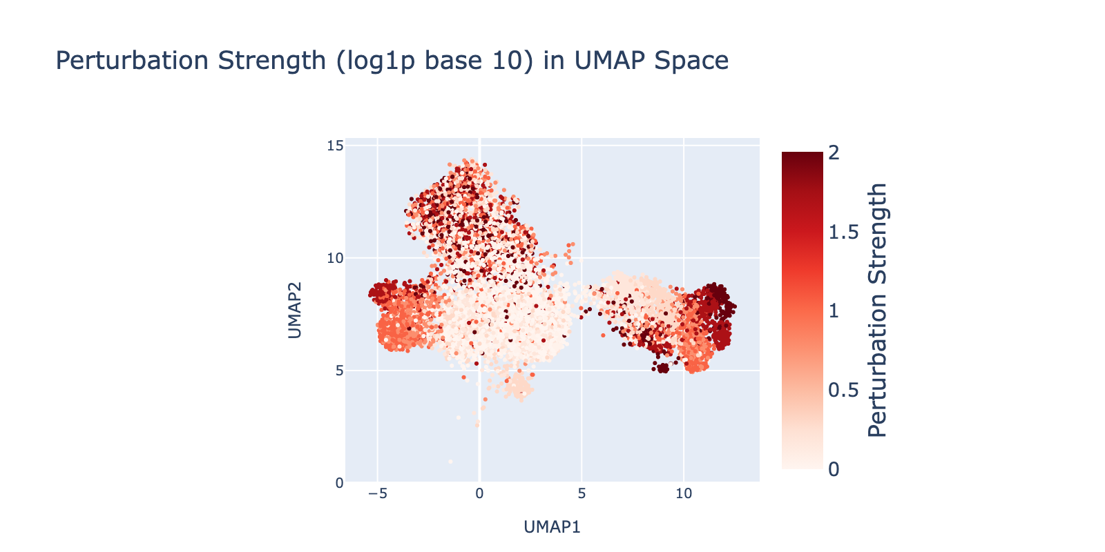
Because perturbation types and doses appear separable, we expected reasonable model performance. Below we show that model outputs track this visual separability and that dose structure is reflected in the learned modules.
Model training {pert}
We framed the task as regression to capture graded perturbation strengths. Targets were dose‑scaled one‑hot vectors (one entry per perturbation) and doses were log‑transformed to stabilize variance.
Model and training settings largely follow the frequency‑regression setup:
- Data:
pertpy.data.srivatsan_2020_sciplex2(). - Features: top 5,000 HVGs (using 10,000 produced strong overfitting).
- Split: 70% train / 30% val; no held‑out test set (exploratory).
- Architecture: bilinear layer; two linear projections $\mathbf{W},\mathbf{V}$ (5k→128) whose elementwise product feeds a linear head $\mathbf{P}$ producing $p$ perturbation outputs. Dropout = 0.4.
- Objective: Huber loss — it outperformed MSE and L1, likely because it is robust to biological outliers.
- Optimizer: Adam, lr = 1e-4, weight decay = 1e-3.
- Schedule: cosine annealing over 100 epochs.
- Batch size: 128.
- Device: CPU; seeds fixed (Python, NumPy, Torch) for reproducibility.
- Biases: including biases did not materially change performance in the original paper or here, so we omitted them to simplify interpretation.
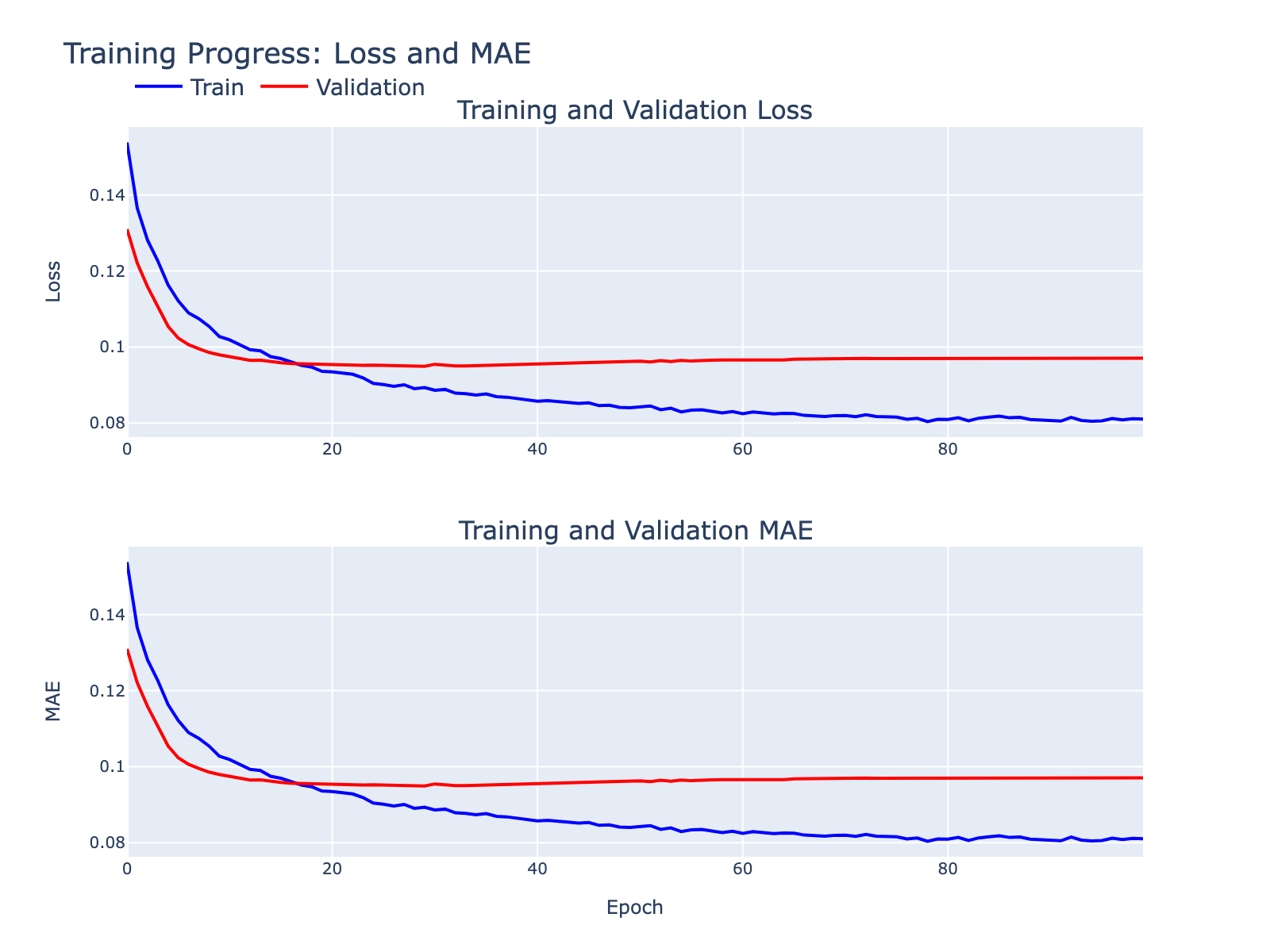
Some overfitting is visible but tolerable for these exploratory goals. We inspected standard diagnostics to summarize model behavior.
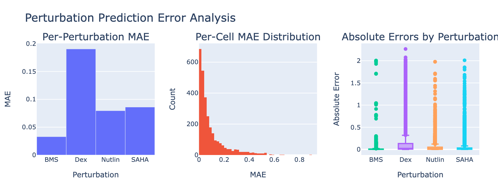
Dex shows a notably high MAE, consistent with its weak or absent dose‑dependent separation in UMAP space.
Model interpretation
As in prior sections, we present one in‑depth example and leave the rest in dropdowns.
SAHA
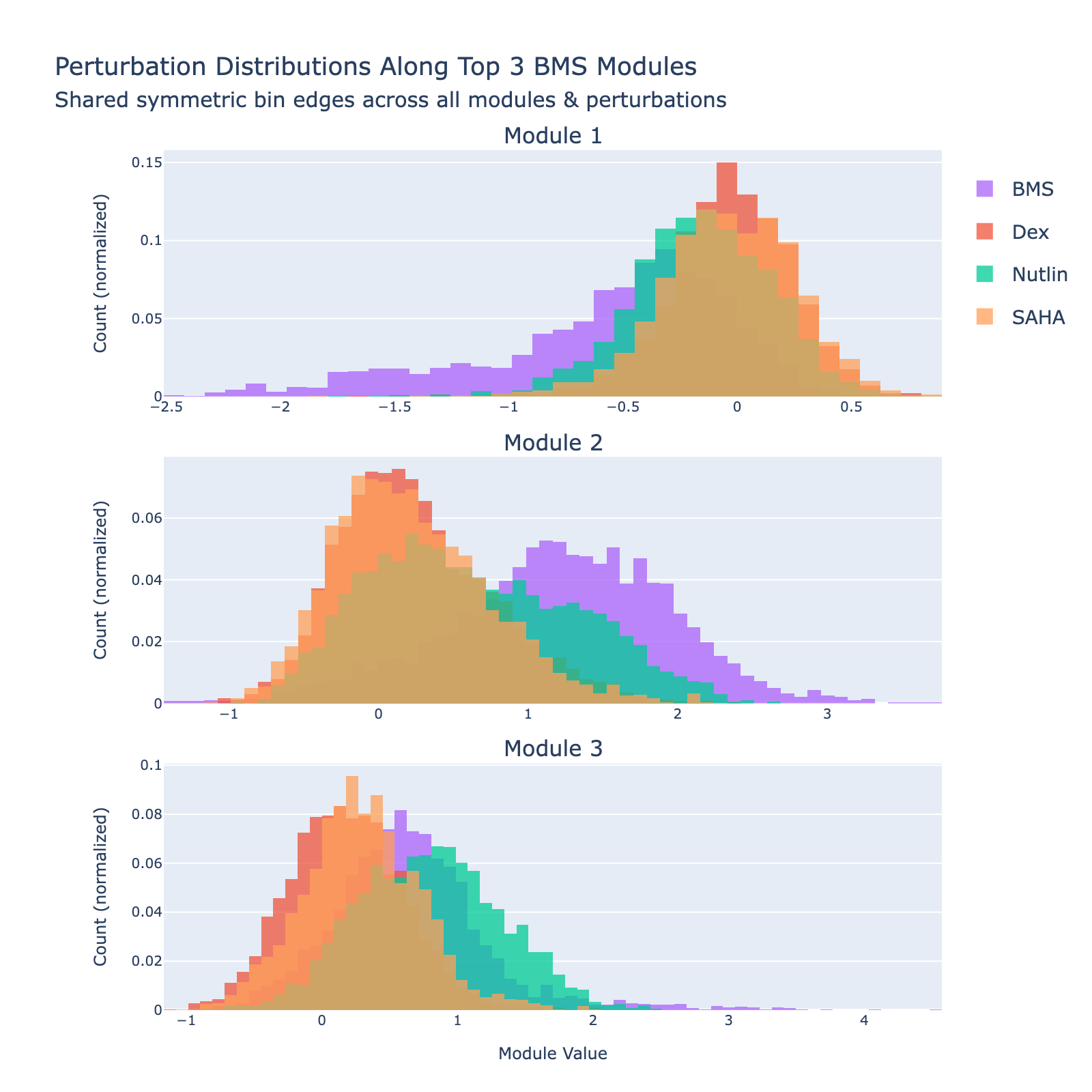
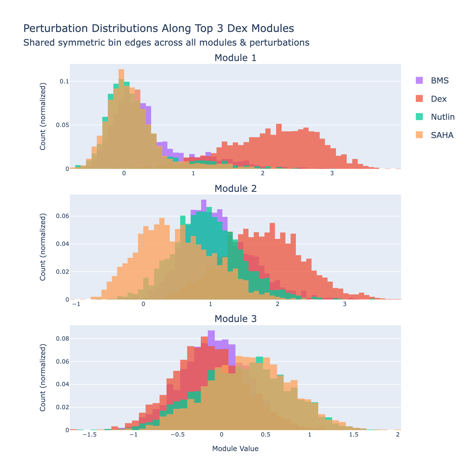
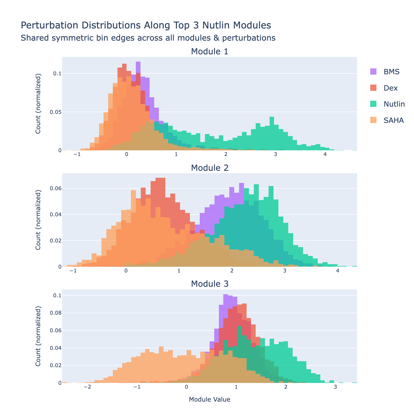
We can also view SAHA from a classification perspective and plot histograms of perturbation labels, analogous to the cell‑type figures above.
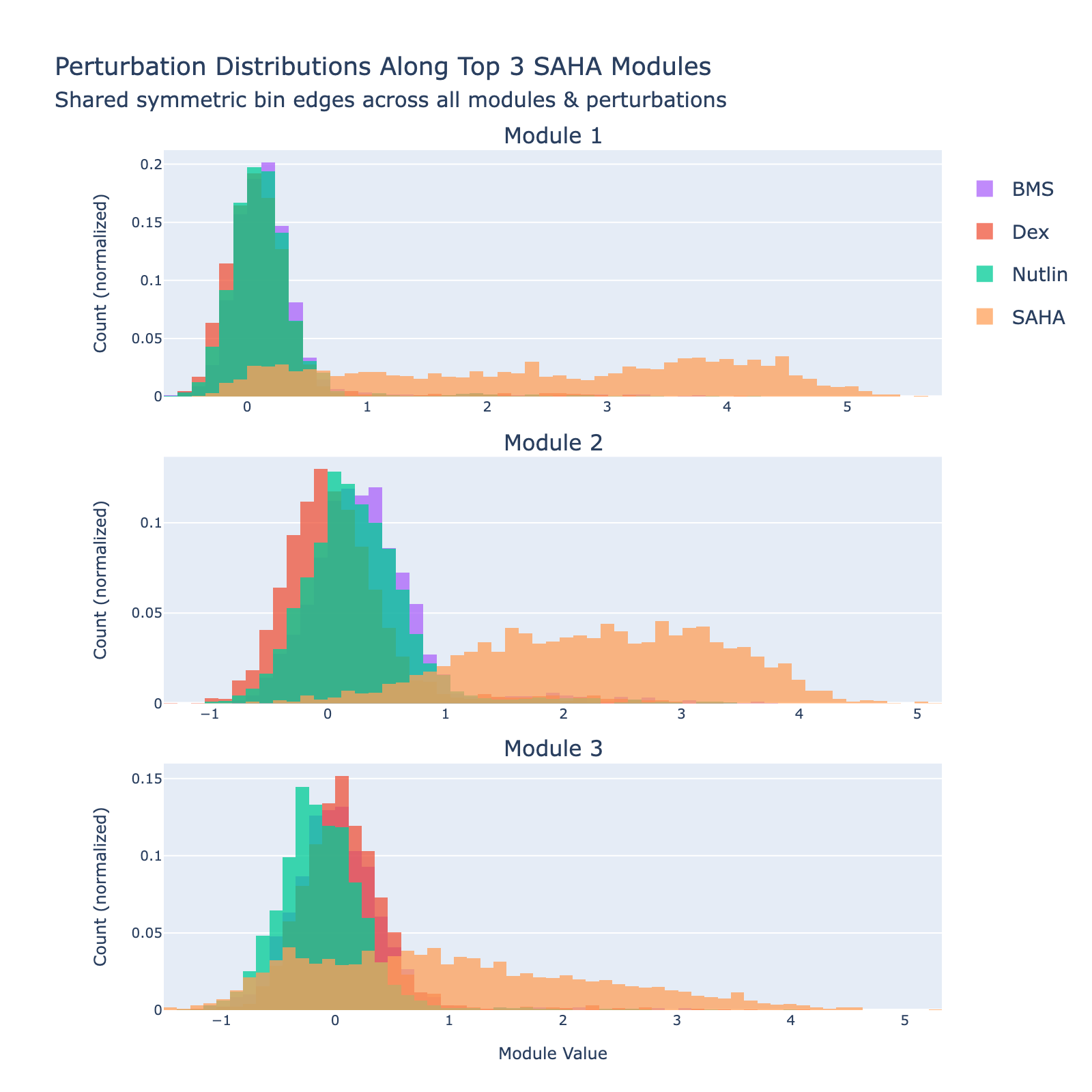
The top three modules each separate SAHA‑treated cells but with distinct distributional signatures.
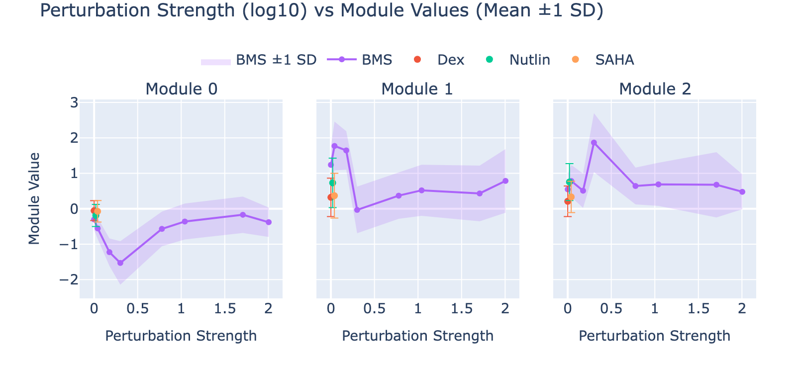
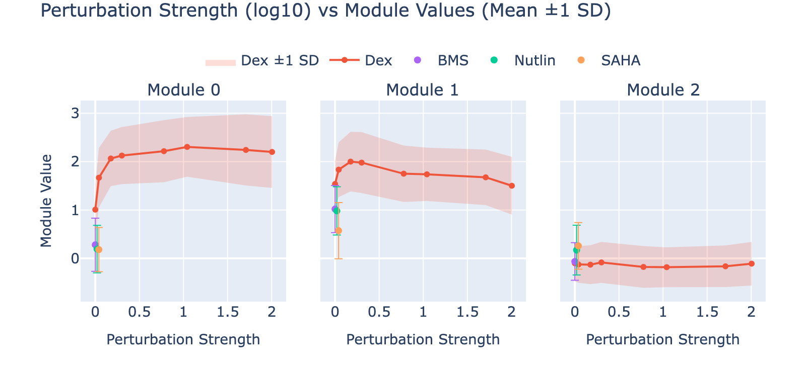
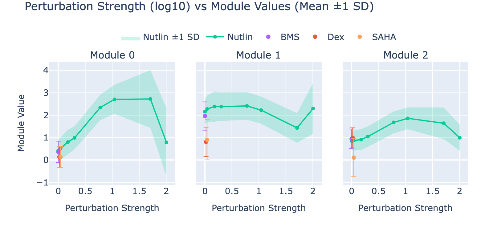
To unpack these, we plot module values by dose. Focusing on module 0, we compute mean ± std for cells labeled as zero‑strength SAHA (which groups non‑SAHA perturbations). These cells cluster near zero. For nonzero SAHA doses the module mean and spread increase, mirroring the frequency analysis and supporting a dose–module correlation.
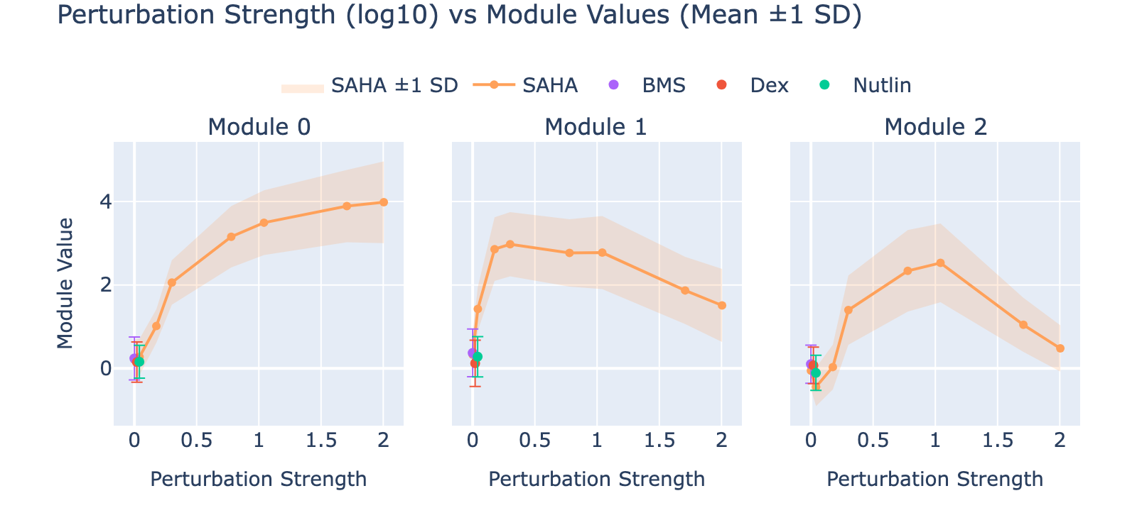
Modules 1 and 2 emphasize low and medium doses respectively, suggesting separable dose‑response components. We inspected eigenvalues to assess their relative importance.

Eigenvalues indicate that modules associated with lower doses explain less variance, though that could reflect task design rather than biology.
Below are the biological notes for module 0.
Overall interpretation
- Positive side: Hypoxia / Myogenesis / Estrogen Response Early enrichments on one pole reflect broad stress, metabolic, and differentiation programs that are suppressed relative to DKK1/lineage‑focused signaling.
- Negative side: Wnt antagonism / differentiation modulation (DKK1) with cardiac‑differentiation regulation terms, suggesting targeted developmental signaling changes under HDAC inhibition.
- Comparison: Contrasts generalized hypoxic/myogenic/estrogenic stress programs with focused Wnt/cardiac differentiation regulation.
Top 10 genes
- Positive: ALDOC, STC1, SMPD3, AC008050.1, RHOB, CKB, NR4A1, ATP1A3, PLA2G4C, ZNF815P
- Negative: FTL, AC025627.1, DKK1, AC078923.1, LINC02045, CRYBG2, RNF103-CHMP3, DNAH12, AC139493.2, LINC01885
Key GO terms
- Positive: Hypoxia; Estrogen Response Early; Myogenesis; TNF‑alpha Signaling via NF‑κB; Estrogen Response Late
- Negative: Negative Regulation of Cardiac Muscle Cell Differentiation; Negative Regulation of Cardiocyte Differentiation; Regulation of Cardiac Muscle Cell Differentiation
This pattern is consistent with known effects of vorinostat (SAHA), a histone‑deacetylase inhibitor that induces chromatin remodeling and dose‑dependent transcriptional reprogramming. The positive pole’s enrichment for stress and inflammatory programs (Hypoxia, TNF‑alpha, estrogen responses) and genes linked to metabolic and differentiation changes aligns with reported SAHA‑induced ER stress, apoptosis, and adaptive responses. The negative pole implicates DKK1 and Wnt antagonism, which is plausible since HDAC inhibition can modulate Wnt/differentiation pathways. Cardiac differentiation terms may reflect pathway crosstalk or dataset‑specific context rather than a direct cardiogenic effect. Overall, the modules capture key molecular hallmarks of SAHA treatment, though experimental follow‑up would be needed to validate pathway‑level claims.
Additional examples
BMS
Overall interpretation
- Positive side: Coagulation / acute inflammatory and nuclear‑receptor responses (fibrin clot factors FGA, FGB, F5; Nuclear Receptors Meta‑Pathway; VEGFA–VEGFR2; TNF‑alpha / EMT) indicating a pro‑thrombotic, stress/remodeling program.
- Negative side: No coherent opposing enrichment (no significant GO terms), suggesting the weight mass is concentrated on the pro‑coagulation/inflammatory direction.
- Comparison: Module represents a unipolar acute‑phase/coagulation plus NF‑κB/EMT axis rather than a balanced contrast.
Top 10 genes
- Positive: DKK1, TP53I3, FAM129A, SREBF1, SEMA3A, ASTN2, Z83843.1, HGD, FKBP5, FGA
- Negative: AC027288.3, PHLDA2, OPCML, ARHGAP15, SERTAD2, AC011287.1, FRMD4A, CATSPERB, AC005614.2, SCUBE3
Key GO terms
- Positive: Blood Clotting Cascade; Common / Formation of Fibrin Clot; Nuclear Receptors Meta‑Pathway; VEGFA–VEGFR2 Signaling; TNF‑alpha Signaling via NF‑κB
- Negative: None significant (p<0.05)
Dex

Overall interpretation
- Positive side: Hypoxia / nuclear‑receptor metabolic adaptation together with keratin/intermediate‑filament cytoskeletal remodeling and angiogenesis/vasculature regulation, pointing to stress‑driven epithelial reprogramming.
- Negative side: No significant opposing enrichment, implying a focused directional module capturing Dex‑induced hypoxia–glucocorticoid responses.
- Comparison: Unipolar activation of glucocorticoid‑responsive metabolic and structural stress pathways.
Top 10 genes
- Positive: COBLL1, ITGB4, MT2A, CIDEC, SDK2, FGD4, FKBP5, TFCP2L1, ANGPTL4, CHST9
- Negative: C5orf66, LINC00824, PHLDA2, PAPLN, CCDC175, PTPRG‑AS1, MT‑ATP6, FAM196A, KCNT2, TCF4
Key GO terms
- Positive: Hypoxia; Nuclear Receptors Meta‑Pathway; Estrogen Response Early; Keratin Filament; Apoptosis
- Negative: None significant (p<0.05)
Nutlin

Overall interpretation
- Positive side: Canonical p53 activation (p53 signaling, DNA damage response, TP53 network, mTORC1) reflecting Nutlin‑induced p53 stabilization and downstream stress programs.
- Negative side: Ion homeostasis and calcium‑handling / cardiac conduction processes, indicating a diminished excitable/ion‑transport state opposite the p53 stress program.
- Comparison: Contrasts p53‑driven apoptotic and metabolic checkpoint activation with reduced calcium/ion signaling pathways.
Top 10 genes
- Positive: MDM2, CDKN1A, FDXR, TP53I3, FAM129A, ALDH3A1, PLD5, LINC01021, TRANK1, AC025627.1
- Negative: USP37, ENOX1, NR0B1, SCUBE3, DPYD, AC016205.1, BX470209.1, PLCXD3, CKB, ROBO2
Key GO terms
- Positive: p53 Signaling Pathway; DNA Damage Response; Genotoxicity Pathway; TP53 Network; mTORC1 Signaling
- Negative: Cell Communication by Electrical Coupling; Calcium Ion Transport Into Cytosol; Ion Homeostasis; Cellular Response to Caffeine; Cardiac Muscle Contraction
Summary {pert}
Our dataset constrained model complexity: including many genes increased overfitting, while very small feature sets reduced biological interpretability. Despite that trade‑off, bilinear MLPs produced perturbation‑specific gene–gene modules that track dose and recover known drug responses, demonstrating a useful balance between predictive performance and transparent, parameter‑based interpretation. Interestingly, several leading modules peak at moderate doses, which suggests separable dose‑dependent components that merit targeted validation.
For next steps, two concrete directions will strengthen and scale these findings. First, evaluate whether linear combinations of output directions can predict responses to perturbation combinations. This tests if learned directions compose meaningfully, as shown in the original bilinear MLP work. Second, build robust out‑of‑sample benchmarks (for example by assembling validation sets from large compendia such as Tahoe‑100M or via cross‑study replication) and explore stronger regularization or structured feature selection (weight decay, sparsity priors, or grouped gene sets) to reduce overfitting while preserving interpretability. Together these efforts would clarify dose‑specific mechanisms and extend the approach to richer, combinatorial perturbation spaces.
Conclusion
Bilinear MLPs offer an interpretable bridge between prediction and mechanism by producing per-output gene–gene interaction matrices whose symmetric eigendecomposition yields readable gene modules. Across tasks the models recovered canonical cell-type markers, captured continuous transcriptional frequencies aligned with developmental trajectories, and revealed dose-dependent perturbation programs tied to model performance. Results are limited by label quality, some overfitting, and the associative nature of weight-based signals, so experimental validation is needed. Future work should test whether output directions compose, build out-of-sample benchmarks, and apply stronger regularization or structured feature selection to reduce overfitting while keeping interpretations usable.